Highway Driving
Drive a car through highway traffic, keeping its lane and overtaking safely with Stanley steering.
Free. Runs in your browser; you'll be asked to sign in first.
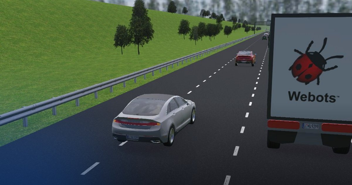
Overview
A Lincoln MKZ drives on a four-lane highway with traffic. In one minute it must cover as much distance as it can without touching another vehicle or the barriers and without entering the emergency lane on the right. The other vehicles are driven by SUMO, a traffic simulator: they accelerate, brake and change lanes on their own.
The lesson builds the three layers of a basic driver-assistance stack: lane keeping with the Stanley steering law, adaptive cruise control (ACC) that turns the measured gap to the car ahead into a safe speed, and a small decision layer that overtakes on the left when the lane is free and returns to the right afterwards.
Theoretical Background
The car and its frame on the road
The car is steered by its front wheels (Ackermann steering). Its pose is described in the road's frame (Frenet coordinates) rather than in world coordinates:
| Symbol | Meaning | Unit |
|---|---|---|
| \(s\) | distance travelled along the road's centre line | m |
| \(d\) | lateral offset of the front axle from the centre line, positive to the left | m |
| \(\psi\) | heading of the car relative to the road's direction, positive to the left | rad |
| \(v\) | forward speed | m/s |
| \(\delta\) | front-wheel steering angle, positive to the left | rad |
The road is 15 m wide with four lanes of width \(w = 3.75\) m. Numbering the three driving lanes from the right (\(i = 0, 1, 2\)), lane \(i\) has its centre at
so \(d_0 = -1.875\) m, \(d_1 = 1.875\) m and \(d_2 = 5.625\) m. The emergency lane lies right of \(d = -w\).
The robot API computes \((s, d, \psi)\) from the GPS (mounted on the front axle), the inertial unit (yaw angle) and a map of the road's centre line, the way an automated car localizes itself on an HD map.
Kinematic bicycle model
At highway speeds the car is well described by the kinematic bicycle model: the two wheels of each axle are merged into one, the wheels roll without slipping, and the wheelbase is \(L = 2.94\) m. Relative to a straight road,
The steering angle sets the curvature \(\kappa = \tan\delta / L\) of the path, and the lateral acceleration felt in the car is \(a_y = v^2\kappa\). At 25 m/s, a steering angle of only 0.05 rad already gives \(a_y \approx 10.6\) m/s\(^2\): on a highway, steering commands are small.
Lateral control: the Stanley law
The Stanley controller (used by Stanford's car that won the 2005 DARPA Grand Challenge) steers the front wheels to cancel two errors at once: the heading error and the cross-track error \(e = d_{\text{ref}} - d\) of the front axle:
clamped to the car's steering range (\(\pm 0.5\) rad here).
- The term \(-\psi\) turns the wheels parallel to the road.
- The term \(\arctan(k e / v)\) points the wheels at a spot on the reference line that lies \(v/k\) metres ahead: the faster the car, the farther ahead it aims and the gentler it steers. For small angles and \(v_s = 0\), the front axle's error obeys \(\dot{e} \approx -k\,e\): it decays exponentially with the time constant \(1/k\), whatever the speed.
- The softening speed \(v_s\) keeps the command finite when the car is (almost) at rest.
A lane change is a jump of \(w = 3.75\) m in the reference. Fed in at once, it would make the car swerve; instead the reference \(d_{\text{ref}}\) moves towards the new lane's centre at a limited lateral rate (1.2 m/s), so a lane change takes about three seconds.
Longitudinal control: adaptive cruise control
The front distance sensor (range 80 m) measures the gap \(g\) to whatever is ahead in the lane. ACC chooses the speed that keeps that gap safe. Two classic rules define "safe":
Constant time gap. The car ahead should be at least \(T\) seconds away, plus a standstill margin \(d_0\):
Solving \(g = g_{\text{safe}}(v)\) for \(v\) gives the speed at which the current gap is just right:
When the car ahead drives at a constant speed, this rule settles exactly at the time gap \(T\) behind it. When the gap shrinks, the target speed drops with it.
Stopping distance. The time-gap rule assumes the car ahead keeps moving. For something standing still (a broken down car, the end of a queue), the car must be able to stop within the free distance. Braking at a constant deceleration \(a\) from speed \(v\) takes the distance \(v^2 / (2a)\), so
is the highest speed from which the car still stops \(d_0\) metres short of the obstacle.
The target speed is the most restrictive of the limits:
With \(d_0 = 8\) m, \(T = 1.5\) s and \(a = 5\) m/s\(^2\), the time-gap term limits the speed in traffic and the stopping term matters at short gaps.
The car's cruise control (the Webots Driver in cruising mode) accelerates towards \(v_{\text{ref}}\) but does not
brake by itself. The brake pedal \(b \in [0, 1]\) is therefore a proportional controller on the over-speed:
Decision making: when to overtake
A car ahead that holds us back (\(v_{\text{ref}} < v_{\max}\)) is a reason to overtake; the rule of the road is to overtake on the left and to return to the right once the road ahead is clear. A lane change is only allowed when the target lane is free next to the car, a little ahead and a little behind it, which the side and diagonal distance sensors tell.
stateDiagram-v2
    [*] --> Keep
    Keep --> ChangeLeft: held back and left lane free
    Keep --> ChangeRight: not held back and right lane free
    ChangeLeft --> Keep: reference reached the new lane
    ChangeRight --> Keep: reference reached the new lane
A minimum time between two lane changes (3 s) keeps the car from hesitating between two lanes.
Task Description
Objective
Implement the functions marked IMPLEMENT HERE in controllers/highway_driving/highway_driving.py:
steering_angle(d_ref, d, psi, speed): the Stanley steering law.safe_speed(front_distance): the ACC target speed, the minimum of \(v_{\max}\), the time-gap speed and the stopping speed.brake_intensity(speed, target_speed): the proportional brake on the over-speed.lane_is_free(distances, ranges, side): whether the lane on one side is free, from the side and diagonal sensors.choose_lane(lane, front_distance, left_free, right_free): overtake on the left, keep right.
The main loop (sense, plan, act), the smooth lane-change reference, the printing and the live plot are given.
System Configuration
- Robot: Lincoln MKZ (Webots
vehicle.Driver), wheelbase 2.94 m, front-wheel steering limited to \(\pm 0.5\) rad. - Sensors:
frontdistance sensor: straight ahead, range 80 m.front left 0/1/2,front right 0/1/2: angled 7.5°, 15° and 22.5° outwards, ranges 20, 15 and 10 m.left,right: sideways, wide beam, range 10 m.rear left,rear right,rear: range 10 m.- GPS on the front axle and an inertial unit, combined with the road map into
get_road_pose()= \((s, d, \psi)\);get_speed()in m/s. - Actuators:
set_cruising_speed(v)[m/s],set_brake(b)[0–1],set_steering_angle(δ)[rad, positive left]. - Environment: a 15 m wide highway with four lanes of 3.75 m; the rightmost is the emergency lane. Straight for the first kilometre, then curves. SUMO traffic at about 50–55 km/h, with a fixed random seed so every run sees the same traffic. A broken-down car with traffic cones stands in lane 1 at about 700 m.
- Control period: 10 ms.
Performance Metrics
The supervisor watches the car's real motion and ends the run after 60 s, on a collision, when the car's centre
enters the emergency lane or leaves the road on the left, or when the car stands still for 10 s. It writes
metrics.json:
| Metric | Meaning |
|---|---|
success |
true when the run lasted the full 60 s without a collision or leaving the lanes and distance_m ≥ 600 m |
ended_reason |
time_limit, collision, entered_emergency_lane, left_the_road, stopped or traffic_not_running |
time_s |
simulated time when the run ended [s] |
distance_m |
distance driven along the road [m] |
average_speed_kmh |
distance_m over time_s [km/h] |
max_speed_kmh |
highest speed reached [km/h] |
lane_changes |
number of times the car moved into another driving lane |
score |
0–100: 100 × distance_m / 1200 m (capped), 0 after a collision or leaving the lanes |
Suggested Algorithm
One control cycle (10 ms):
- Sense: read the speed \(v\), the road pose \((s, d, \psi)\) and all distance sensors.
- Lane keeping: compute \(\delta\) with the Stanley law towards the current reference \(d_{\text{ref}}\).
- ACC: compute \(v_{\text{ref}}\) from the front gap and the brake from the over-speed.
- Decide: when the last lane change is over and has been held for 3 s, check both sides and choose the lane.
- Reference: move \(d_{\text{ref}}\) towards the chosen lane's centre at 1.2 m/s.
- Act: send the cruising speed, the brake and the steering angle.
Validation Checklist
- The car stays centred in its lane: \(|d - d_{\text{ref}}|\) stays below about 0.1 m on the straight and \(\psi\) near 0.
- Behind a slower car, the speed settles at the speed of the car ahead and the gap near \(d_0 + Tv\) (the plot's dashed line); the brake is used only when the gap closes quickly.
- On a free road the car accelerates to \(v_{\max}\) (90 km/h) and moves back to the right.
- Lane changes start only when the side sensors see nothing, take about three seconds and do not overshoot.
- The car never enters the emergency lane and finishes the minute without a collision.
The live plot (Visualization tab) shows the speed and the safe speed, the gap and the safe gap, and the lateral
offset with its reference. Set SHOW_PLOT = False to run without it.
References
- Webots automobile library: the Driver API
- Webots SUMO interface
- G. M. Hoffmann, C. J. Tomlin, M. Montemerlo, S. Thrun, "Autonomous Automobile Trajectory Tracking for Off-Road Driving: Controller Design, Experimental Validation and Racing", American Control Conference 2007 (the Stanley law).
- R. Rajamani, Vehicle Dynamics and Control, Springer, 2nd ed. 2012: chapter 2 (bicycle model) and chapters 5–6 (cruise control and adaptive cruise control).
- Adaptive cruise control on Wikipedia.
Extension Ideas
- Estimate the closing speed \(\dot{g}\) from successive gap readings and add it to the ACC law (\(a = k_1 (g - g_{\text{safe}}) + k_2 \dot{g}\)), so the car brakes earlier for a much slower car.
- Replace the map-based lane offset with lane detection from the car's
camera: find the lane lines in the image and estimate \(d\) and \(\psi\) from them. - Tune \(v_{\max}\), \(T\) and the lane-change rules for more distance without losing safety, then try another traffic seed in the supervisor.