Inverted Pendulum Control
Keep a pole upright on a moving e-puck by tuning a PID controller on the pendulum's angle.
Free. Runs in your browser; you'll be asked to sign in first.
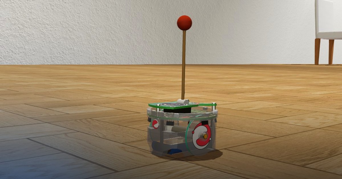
Inverted Pendulum
Overview
An e-puck carries a pendulum on a free hinge: a light pole with a 50 g ball at its top. The pendulum falls unless the robot keeps driving its wheels under it, the way you balance a broom on your hand. A supervisor pushes the ball with a random force that grows with time, so sooner or later every controller loses; the goal is to keep the pendulum up as long as possible.
The controller is a PID loop that is already written: it reads the pendulum angle and sets the wheel speed. The lesson is about tuning it: what \(K_P\), \(K_I\) and \(K_D\) do on this particular plant, why the textbook recipe does not apply directly, and how to read the console to see what the loop is doing.

Theoretical Background
The Pendulum on a Moving Base
Model the pendulum as a point mass at distance \(l\) from the hinge, and let the robot (the hinge) accelerate along the ground with acceleration \(a\). For a small angle \(\theta\) from the vertical, the pendulum obeys
| Symbol | Meaning | Value here |
|---|---|---|
| \(\theta\) | pendulum angle from the vertical | rad, \(0\) = upright |
| \(l\) | distance from the hinge to the ball | \(\approx 0.08\) m |
| \(g\) | gravity | \(9.81\) m/s² |
| \(a\) | acceleration of the robot | m/s² |
| \(d(t)\) | the supervisor's push, as an acceleration | random, grows with time |
Without control (\(a = 0\)) the solution grows like \(e^{t\sqrt{g/l}} \approx e^{11t}\): a small tilt doubles about every 0.06 s. The only way to bring the ball back is to accelerate the base towards the side it leans to.
What the Controller Commands
The controller does not set an acceleration, it sets a wheel speed \(\omega\) (rad/s); the robot's speed is \(v = r\omega\), with wheel radius \(r \approx 0.0205\) m. With the angle as the error, \(e = \theta\), the PID output is
In the code, one step of length \(\Delta t\) (robot.dt, 4 ms) updates the integral with the trapezoid rule and the
derivative with a finite difference:
so the integral is in rad·s and the derivative in rad/s, and the gains carry the units that turn them into a wheel speed: \(K_P\) in (rad/s)/rad, \(K_I\) in (rad/s)/(rad·s), \(K_D\) in (rad/s)/(rad/s).
The Closed Loop
Because the output is a speed, the acceleration that balances the pendulum is its derivative: \(a = r\dot{\omega} = r\,(K_P\dot{\theta} + K_I\theta + K_D\ddot{\theta})\) (assuming the motors follow the commanded speed quickly). Putting it into the pendulum equation gives
a mass-spring-damper, in which each gain plays a different part from the usual one:
| Gain | Role in this loop | Too low | Too high |
|---|---|---|---|
| \(K_I\) | the stiffness: pushes the pendulum back to upright | below \(g/r \approx 480\) it cannot beat gravity and the pendulum falls | stiff and fast: little damping, it shakes and falls |
| \(K_P\) | the damping: slows the swing down | oscillations that grow under the pushes | sharp reactions to every small change of angle |
| \(K_D\) | adds inertia (\(l + rK_D\)): slows the whole loop down | (it may be zero) | sluggish, the pushes win |
The loop is stable when all three coefficients are positive: \(K_I > g/r\), \(K_P > 0\) and \(K_D > -l/r\). Its natural frequency and damping ratio are
With the provided gains (\(K_P = 100\), \(K_I = 5000\), \(K_D = 1\)): \(\omega_n \approx 30\) rad/s and \(\zeta \approx 0.34\). A proportional-only controller (\(K_I = 0\)) has no stiffness at all and drops the pendulum in under a second: here the integral term does the main work, unlike in most PID loops.
Why Every Controller Loses Eventually
The integral term is, up to a factor, the robot's speed: to stay under the pendulum, the robot has to absorb every push by changing its speed, and nothing in this loop brings the speed back to zero. The pushes are random, so the speed wanders like a random walk, and the pushes grow with time. The e-puck's wheels turn at most 6.28 rad/s (about 0.13 m/s): once the controller asks for more, the motors saturate, the base can no longer accelerate, and the pendulum falls within a fraction of a second. On the console this shows as the wheel speed creeping towards \(\pm 6.28\) rad/s before the fall. Good gains delay that moment; only a different controller (see Extension Ideas) can push it further.
Task Description
Objective
Tune the PID controller in controllers/inverted_pendulum/inverted_pendulum.py to keep the pendulum upright as long as
possible:
- Run the provided gains and read the console: the angle, the integral and the wheel speed command every 0.5 s (the motors clamp it to \(\pm 6.28\) rad/s).
- Change
KP,KIandKDone at a time and compare the balancing time over several runs (the pushes are random, so one run proves little). - Explain your best gains with the closed-loop model above: the stiffness, the damping, and when the wheels saturate.
System Configuration
- Robot: e-puck differential-drive robot, both wheels driven with the same speed.
- Sensor: the pendulum's hinge position sensor (
get_pendulum_position(), rad, \(0\) = upright, resolution \(10^{-5}\) rad); the hinge stops at \(\pm 1.6\) rad. - Actuators: left and right wheel motors (
set_wheel_velocity(left, right), rad/s, clamped to \(\pm 6.28\) rad/s). - Pendulum: a 50 g ball about 0.08 m above the hinge, starting 0.05 rad from the vertical.
- Control period:
robot.dt= 4 ms (the world's basic time step). - Disturbance: every step, the supervisor pushes the ball with a force of \(0.01 \cdot U(-1, 1) \cdot t\) N, where \(t\) is the simulated time in seconds and \(U(-1, 1)\) a uniform random number.
Performance Metrics
The supervisor ends the run when the pendulum's angle exceeds 1.5 rad (it has fallen), writes metrics.json and
pauses the simulation.
| Metric | Meaning |
|---|---|
time |
simulated time the pendulum stayed up [s]; higher is better |
Because the pushes are random, compare gains by the typical result of several runs. The provided gains balance for between about 6 and 17 s, 10 to 11 s on average.
Suggested Algorithm
At each control step:
- Read the pendulum angle \(\theta_k\).
- Add the trapezoid \(\frac{\theta_k + \theta_{k-1}}{2}\Delta t\) to the integral.
- Compute the derivative \((\theta_k - \theta_{k-1}) / \Delta t\).
- Compute the wheel speed \(\omega = K_P\theta_k + K_I I_k + K_D D_k\) and remember \(\theta_k\) for the next step.
- Drive both wheels with the same speed (the sign in the code makes the robot move towards the side the pendulum leans to).
A tuning procedure that follows from the closed-loop model:
- Make the loop stiff enough: \(K_I\) well above \(g/r \approx 480\) (e.g. 2000 to 6000). With \(K_P = 0\) there is no damping, and the pendulum oscillates and falls within a couple of seconds.
- Increase \(K_P\) until the swing after the start dies out quickly (\(\zeta\) around 0.3 to 0.7).
- Raise \(K_I\) to make the loop faster, raising \(K_P\) with it to keep the damping.
- Try a small \(K_D\) and keep it only if the average time improves.
Validation Checklist
- The pendulum settles near upright within the first second.
- The console's angle stays within a few hundredths of a radian while the pushes are small.
- The wheel speed stays well inside \(\pm 6.28\) rad/s for the first seconds and approaches the limit only before the fall.
- The average balancing time over several runs is at least that of the provided gains.
References
- PID controller
- Inverted pendulum
- E-puck robot (Webots documentation)
- K. J. Åström, R. M. Murray, Feedback Systems, chapter 10 (PID control), Princeton University Press, 2008.
Extension Ideas
- Bring the speed back towards zero: lean the pendulum's target against the motion, i.e. use the error \(e = \theta + c\,\omega\) in the integral, with the previous step's wheel speed \(\omega\) and a small \(c\) (about 0.001 to 0.0015 s). The robot then brakes before its wheels saturate; with the provided gains this keeps the pendulum up about 30% longer. Find the sign and size of \(c\) yourself: too much makes it fall at once.
- Plot the angle and the wheel speed over time with Matplotlib and watch the speed's random walk.
- Replace the PID with a state-feedback controller (LQR) on the angle, its rate and the robot's speed.