Obstacle Avoidance
Steer a Thymio through a cluttered classroom using its proximity sensors, without bumping into anything.
Free. Runs in your browser; you'll be asked to sign in first.
Overview
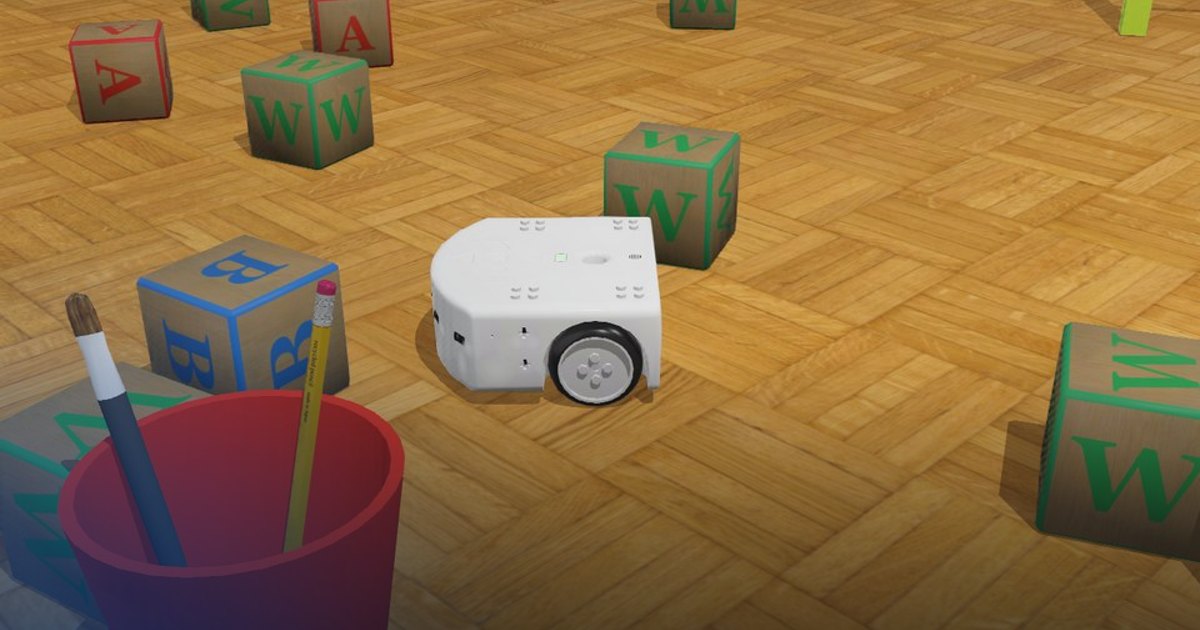
A Thymio II starts at one end of a classroom and must reach the finish line at the other end, about 6 m away. The floor in between is cluttered: letter blocks, a ball, a pen pot, chair and table legs, and a dozen cubes that the supervisor drops at random at the start of every run, so no two runs are the same and no path can be learned by heart. The robot has no map: it only feels what lies a few centimetres in front of it with five infra-red proximity sensors, and knows which way it faces from a compass.
The lesson teaches reactive control: wheel speeds computed directly from the current sensor readings, without a map or a plan. You will build a Braitenberg vehicle (a weighted sum of sensor activations per wheel), add a goal-seeking heading controller, blend the two through the differential-drive kinematics, and wrap everything in a two-state machine that backs the robot out of situations the weighted sum cannot handle.
Theoretical Background
Infra-red proximity sensors
Each of the Thymio's front sensors emits infra-red light and measures how much is reflected back. The closer the obstacle, the stronger the reflection, so the reading \(s_i\) falls with the distance \(d\):
| distance \(d\) | 0 cm | 2 cm | 4 cm | 6 cm | 8 cm | 9 cm | > 9.3 cm |
|---|---|---|---|---|---|---|---|
| reading \(s_i\) | 4235 | 4139 | 2965 | 2248 | 1597 | 1195 | 0 |
Three properties matter for control:
- Short range. Nothing farther than about 9 cm is seen. At \(0.14\ \text{m/s}\) the robot covers that range in 0.65 s, so the controller must react within a few control steps.
- Narrow rays. The sensors point at \(+40^\circ, +20^\circ, 0^\circ, -20^\circ, -40^\circ\) from the robot's heading (positive to the left), and each one measures along a single line. A thin object, or the corner of a box, can sit between two rays and stay unseen until it touches the robot; and an obstacle beside the robot is never seen at all.
- Colour. The reflected light depends on the surface: in Webots, as on the real robot, light and red obstacles return more than dark and non-red ones, so a dark object is seen later, closer to the robot.
The controller works with activations, the readings normalised to \([0, 1]\):
so \(a_i = 0\) means "nothing within range" and \(a_i \approx 1\) means "touching".
Braitenberg vehicles
Valentino Braitenberg showed (Vehicles, 1984) that wiring sensors straight to motors produces behaviour that looks purposeful. With \(n\) sensors, each wheel speed is a constant plus a weighted sum of the activations:
or, in matrix form, \(\boldsymbol{\omega} = \boldsymbol{\omega}_0 + W \mathbf{a}\) with \(W \in \mathbb{R}^{2 \times 5}\). To avoid obstacles (Braitenberg's "fear"), a sensor on the left must speed up the left wheel and slow down the right one, so the robot turns right, away from it; a sensor on the right does the opposite. The weights of this lesson, in rad/s per unit of activation:
| sensor | outer left | left | centre | right | outer right |
|---|---|---|---|---|---|
| \(W_L\) (left wheel) | +6 | +10 | +4 | −14 | −10 |
| \(W_R\) (right wheel) | −10 | −14 | −4 | +10 | +6 |
The inner sensors weigh more than the outer ones because an obstacle near the robot's centre line is more urgent than one off to the side. The centre sensor turns the robot right: a perfectly symmetric vehicle facing an obstacle head-on would have no reason to prefer a side, and this asymmetry breaks the tie. Its weight is smaller than the side sensors', so an obstacle seen by the centre and a right sensor still turns the robot left. Braking is left to the forward speed (below), not to the weights: if the centre sensor slowed both wheels, the robot would settle at the distance where the braking cancels the forward drive and stay there, a deadlock.
A Braitenberg vehicle as a whole is a linear map from activations to wheel speeds, so it is easy to analyse: the robot's turn rate is \(\omega = \frac{r}{d}\,(W_R - W_L)\,\mathbf{a}\), here \(\frac{r}{d}\,[-16,\ -24,\ -8,\ +24,\ +16]\,\mathbf{a}\), negative (clockwise, to the right) for obstacles on the left and the centre.
Differential-drive kinematics
The Thymio has two wheels of radius \(r = 0.021\) m, \(d = 0.0935\) m apart. Its forward speed \(v\) and turn rate \(\omega\) (counter-clockwise positive) follow from the wheel speeds \(\omega_L, \omega_R\):
Inverting the two equations gives the wheel speeds that produce a wanted motion \((v, \omega)\):
This lets each behaviour be designed in the robot's natural terms (go this fast, turn this fast) and converted to wheel commands at the end.
Goal seeking with a heading controller
Avoiding obstacles alone makes the robot wander; it also has to make progress. The finish line lies along the world's \(+y\) axis, i.e. at the heading \(\theta_g = \pi/2\). With the measured heading \(\theta\), a proportional controller turns the robot back towards the goal:
Wrapping makes the robot turn the short way round (an error of \(+350^\circ\) is really \(-10^\circ\)), and the saturation keeps a large error from producing a violent spin.
The compass reports the direction of north (\(+y\)) in the robot's frame, \((\sin\theta, \cos\theta)\), so
\(\theta = \operatorname{atan2}(n_x, n_y)\); robot.py does this for you.
Blending the behaviours
Goal seeking and avoidance pull in different directions near an obstacle. The controller blends them by letting the obstacle win as it gets closer:
The forward speed \(v_c\) drops as the nearest obstacle gets closer, and the goal's turn rate is scaled by an obstacle memory \(m \in [0, 1]\). The memory is needed because an obstacle that leaves the sensors' view after a turn is usually right beside the robot, not gone; if the goal pulled at full strength at once, it would steer the robot straight back into it. The memory is 1 while any sensor sees something and fades linearly over \(T_m = 1.5\) s afterwards:
so the goal regains its full pull only after the robot has driven about \(v_c T_m \approx 20\) cm past the last obstacle.
This is the potential-field idea in its simplest form: the goal attracts, obstacles repel, and the robot follows the sum. It inherits the method's weakness too: where attraction and repulsion cancel (a dead end facing the goal), the robot can get stuck in a local minimum.
A two-state machine for the hard cases
A weighted sum reacts in proportion; it cannot decide "this is too close, back off". A small state machine adds that decision:
stateDiagram-v2
    [*] --> FORWARD
    FORWARD --> ESCAPE: max activation > 0.6 (about 5 cm)
    ESCAPE --> FORWARD: escaped for 0.6 s and every activation < 0.6
    FORWARD: FORWARD - goal seeking + Braitenberg
    ESCAPE: ESCAPE - reverse and turn away
On entering ESCAPE the robot picks the side that sees less (left sensors \(a_0 + a_1\) against right sensors \(a_3 + a_4\)) and reverses slowly while turning towards it. Reversing matters: the Thymio's front reaches 8 cm ahead of its wheel axle, so spinning in place next to an obstacle swings the nose into it.
Task Description
Objective
Implement the functions marked IMPLEMENT HERE in controllers/avoid_obstacles/avoid_obstacles.py:
get_activations(raw_values): normalise the five readings to activations in \([0, 1]\).update_obstacle_memory(memory, activations, dt): the obstacle memory \(m_k\), 1 while something is seen, then fading.goal_turn_rate(heading): the saturated proportional heading controller \(\omega_g\).unicycle_to_wheels(v, w, r, d): the inverse differential-drive kinematics.braitenberg(activations): the wheel-speed corrections \(W \mathbf{a}\).choose_state(state, activations, time_in_state): the FORWARD / ESCAPE transitions.
The main loop that calls them (Sense, Plan, Act) is given; read it to see how the pieces fit together, then tune the constants at the top of the file.
System Configuration
- Robot: Thymio II (Mobsya), a differential-drive robot about 11 cm wide, wheel radius 0.021 m, axle 0.0935 m.
- Sensors:
prox.horizontal.0…prox.horizontal.4: the five front infra-red proximity sensors, left to right, at \(+40^\circ, +20^\circ, 0^\circ, -20^\circ, -40^\circ\); readings 0 (nothing within 9.3 cm) to about 4300 (touching).compass: in the body slot;robot.get_heading()turns it into the heading in rad (\(\pi/2\) faces the finish).- Actuators:
motor.left,motor.right, velocity-controlled, at most 9.53 rad/s (about 0.20 m/s). - Environment: a 7.8 m × 9.8 m classroom. The robot starts at \((0, -2.68)\) facing \(+y\); the finish line is at \(y = 3.3\) m. Fixed obstacles and 13 cubes dropped at random in \(x \in [-0.5, 1.1]\), \(y \in [-1, 1]\) m.
- Control step: 16 ms.
Performance Metrics
The supervisor (controllers/supervisor) watches the robot's real position and the contacts of its body. A
collision is the body touching anything above 2 cm from the floor; contacts less than 0.5 s apart count as one.
The run ends when the robot crosses the finish line, at its third collision, when it has moved less than 5 cm in 10 s
(stuck, or the controller stopped), or after 80 s. It then writes
metrics.json:
| metric | unit | meaning |
|---|---|---|
success |
bool | the robot crossed \(y = 3.3\) m with fewer than 3 collisions within 80 s |
time |
s | simulated time when the run ended |
progress |
0..1 | the farthest the robot got towards the finish line, as a fraction of the 5.98 m |
distance_m |
m | length of the path the robot drove |
collisions |
count | collisions with obstacles |
score |
0..100 | \(60 \cdot \text{progress} + 40 \cdot \frac{80 - t}{80}\) (the time bonus only on success) \(- 10 \cdot \text{collisions}\) |
A clean, quick run (no collisions, finish in 45 s) scores about 77.
Suggested Algorithm
At each control step:
- Sense: read the five proximity sensors and normalise them into activations; read the heading.
- Update the obstacle memory.
- Plan: update the state machine (FORWARD or ESCAPE).
- In FORWARD: compute the goal turn rate, scale it by \(1 - m\), scale the cruise speed by \(1 - \max_i a_i\), convert \((v, \omega)\) to wheel speeds and add the Braitenberg corrections.
- In ESCAPE: convert a slow reverse speed and a turn away from the more crowded side to wheel speeds.
- Act: send the wheel speeds (
robot.pyclamps them to ±9.53 rad/s).
Validation Checklist
- With nothing in front, the activations print as zeros and the robot drives straight towards the finish line.
- Holding an obstacle on the robot's left makes it turn right, and the other way round.
- A head-on obstacle makes the robot slow down and veer, or back off in ESCAPE, rather than push into it.
- After passing an obstacle the robot turns back to a heading of about 90° within a second or two.
- The console shows few ESCAPE events, and the supervisor reports zero or one collision on most runs.
- Several runs in a row succeed: the cubes land differently every time.
References
- Thymio II in Webots
- Webots DistanceSensor (infra-red sensors and lookup tables)
- Braitenberg vehicle, and V. Braitenberg, Vehicles: Experiments in Synthetic Psychology, MIT Press, 1984
- R. Siegwart, I. Nourbakhsh, D. Scaramuzza, Introduction to Autonomous Mobile Robots, 2nd ed., MIT Press, 2011: §3.2 (wheel kinematics) and §6.4 (obstacle avoidance)
- R. C. Arkin, Behavior-Based Robotics, MIT Press, 1998 (blending behaviours, potential fields)
Extension Ideas
- Raise
V_CRUISEtowards the motors' 0.20 m/s and retune the weights: how fast can the robot go before the 9 cm sensor range is no longer enough? - Replace the fixed escape direction with a turn towards the goal side when both sides are equally crowded, and count how often the robot gets stuck in a local minimum.
- Make the weights depend on speed (react earlier when going faster), or learn them: run many episodes and keep the weight matrix with the best average score.