Line Following with Localization
Follow a line with an e-puck while estimating its pose from wheel odometry.
Free. Runs in your browser; you'll be asked to sign in first.
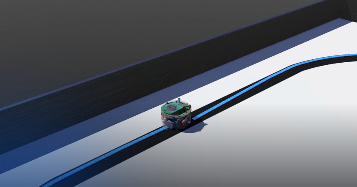
Line Following with Odometry
Overview
In this lesson, the robot follows a floor line while also estimating its pose from wheel encoder data. The robot must keep the line under control and, at the same time, maintain an estimate of its own position and heading.
The lesson combines reactive line following with encoder-based pose estimation.
Theoretical Background
Line Following
A simple line follower uses the ground sensors to decide whether the robot should move forward, turn left, or turn right.
Odometry Localization
Odometry estimates motion by integrating wheel rotations over time.
For a differential-drive robot, the wheel angular speeds are computed from the encoder increments:
The robot linear and angular speeds are then:
where \(R\) is the wheel radius and \(D\) is the distance between the wheels.
A simple pose update is:
Odometry provides a running pose estimate without external position sensors, but it also accumulates drift over time.
Task Description
Objective
Implement four functions in line_following_with_localization.py:
get_line_following_speeds(line_left, line_right, max_speed): the wheel speeds that keep the robot on the line (turn toward the side where only one sensor sees the line, otherwise drive straight).get_wheels_speed(encoder_values, old_encoder_values, dt): the wheel angular speeds from the encoder increments.get_robot_speeds(wl, wr, r, d): the robot's linear speed \(u\) and angular speed \(\omega\).get_robot_pose(u, w, x_old, y_old, phi_old, dt): the integrated pose, with the heading wrapped to \([-\pi, \pi)\).
The main loop calls them in this order and prints the estimated pose about twice a second.
System Configuration
- Robot: e-puck differential-drive robot (wheel speeds up to about 6.28 rad/s)
- Sensors: wheel encoders (
get_wheel_encoder_positions(), rad) and three ground sensors,gs0(left),gs1(centre) andgs2(right); a reading below 600 means the sensor sees the dark line - Actuators: left and right wheel motors
- Parameters: wheel radius \(R = 0.020\) m, wheel separation \(D = 0.057\) m (the values in the code)
- Initial pose:
get_current_pose()gives the true starting pose once, to initialise the estimate - Environment: a closed oval of dark line (about 4.7 cm wide) on a bright floor; the robot starts on the line
Performance Metrics
A supervisor follows the robot's real position and compares it with the centre of the painted line. The run ends
after one full lap, when the robot is more than 10 cm from the line for 5 s (line_lost), when it stops moving for
5 s (stopped), or after 90 s. It writes:
| Metric | Meaning |
|---|---|
success |
one lap completed, on the line at least 90% of the time |
ended_reason |
lap_completed, line_lost, stopped or time_limit |
time_s |
simulated time of the run [s] |
laps |
laps driven along the line |
distance_m |
path length of the robot [m] |
average_speed_m_s |
distance_m / time_s [m/s] |
mean_line_error_m, max_line_error_m |
distance from the robot's centre to the line's centre [m] |
on_line_ratio |
fraction of the time within 4 cm of the line's centre |
score |
0 to 100: 100 * min(1, laps) * on_line_ratio |
The odometry is not graded: check it in the console. After one lap the robot is back near its starting point, so the printed pose should be close to the initial one; the difference is the accumulated drift.
Suggested Algorithm
At each control step:
- Read the ground sensors and choose wheel commands for line following.
- Apply the wheel commands.
- Read the wheel encoder positions.
- Compute the wheel angular speeds.
- Compute the robot linear and angular speeds.
- Integrate the pose estimate.
- Print or log the estimated pose.
Validation Checklist
- Straight motion changes position mainly along the current heading.
- Turning produces a nonzero angular speed estimate.
- The heading stays bounded to a wrapped angular range.
- The pose estimate updates once per control cycle.
- The robot continues to follow the line while odometry runs in parallel.
References
Extension Ideas
- Add the center ground sensor for more precise line tracking.
- Plot the estimated pose over time to study odometry drift.
- Add a correction source such as a compass, GPS, or landmark detector.