Robot Programming
Write your first controller: drive a Thymio exactly 25 cm forward and stop on the target.
Free. Runs in your browser; you'll be asked to sign in first.
Robot Programming: Drive to a Target and Stop
Overview
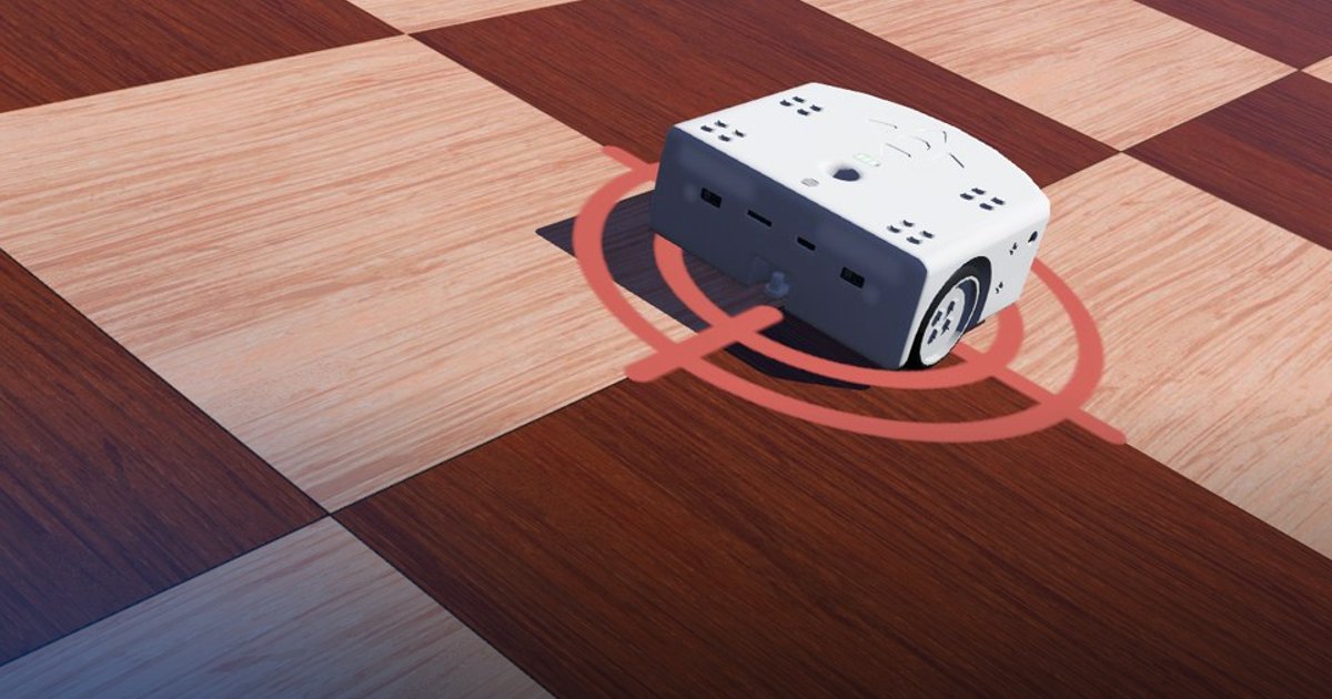
The Thymio II starts at the centre of the arena, facing a target square 0.25 m straight ahead. The robot must drive to the target and stop on it: no turns, no obstacles, just the two wheels and their encoders.
This first lesson covers the basics every later lesson builds on: the control loop that runs once per simulation step, commanding a wheel motor by its angular speed, converting between wheel rotation and distance travelled, and using a measurement (odometry) instead of a timer to decide when to stop.
Theoretical Background
The control loop
A Webots controller is a loop. Each call to robot.step() advances the simulated world by one time step
\(\Delta t\) (here \(\Delta t = 20\) ms), after which the controller reads its sensors, decides, and sends new commands
that hold until the next step. Every control program in this course has the same three phases:
graph LR
    S[Sense: read the encoders] --> P[Plan: choose a speed]
    P --> A[Act: set the wheel speeds]
    A --> T[step: advance the simulation by dt]
    T --> S
Wheel speed and robot speed
The Thymio II is a differential-drive robot: two motorised wheels on a common axle and a passive support. Its motors are used in velocity mode: the command is the wheel's angular speed \(\omega\) in rad/s, and the motor controller keeps the wheel turning at that speed (up to \(\omega_{max} = 9.53\) rad/s).
A wheel of radius \(r\) that rolls without slipping moves its axle forward by the length of the arc it unrolls: one radian of rotation moves it \(r\) metres. So the wheel's linear speed \(v\) and its angular speed \(\omega\) are related by
When both wheels turn at the same speed, the robot drives straight at that linear speed. When they differ, it turns; later lessons use the full differential-drive model \(v = \frac{r}{2}(\omega_r + \omega_l)\), \(\dot\phi = \frac{r}{D}(\omega_r - \omega_l)\), with \(D\) the distance between the wheels.
| Symbol | Meaning | Value |
|---|---|---|
| \(r\) | wheel radius | 0.021 m |
| \(\omega_{max}\) | maximum wheel angular speed | 9.53 rad/s |
| \(v_{max}\) | top speed, \(r\,\omega_{max}\) | 0.20 m/s |
| \(\Delta t\) | control step | 0.020 s |
| \(d^*\) | distance to the target | 0.25 m |
Open loop: stopping by the clock
The simplest plan is to drive at a constant speed \(v\) for a time \(T = d^*/v\) and then stop: at 0.10 m/s, for 2.5 s. This is open-loop control: the robot never checks where it is. It fails as soon as the model is wrong: the motors need time to accelerate, the wheel radius is not exactly 0.021 m, wheels slip, the battery sags on a real robot. Every such error ends up, unseen, in the final position.
Closed loop: odometry
A better plan measures the progress. Each wheel has an encoder (a position sensor) that reports the wheel's angle \(\theta\) in radians. If the left and right wheels have turned by
since the start, each wheel has rolled \(r\,\Delta\theta\) metres, and the centre of the robot, halfway between them, has travelled
Estimating motion by integrating wheel rotations is called odometry. Averaging the two wheels keeps the estimate right even when one wheel turns slightly more than the other. The remaining distance \(e(t) = d^* - d(t)\) is the error the controller drives to zero.
Slowing down: a proportional speed profile
Driving at full speed until \(e < \varepsilon\) and then stopping overshoots: in one step the robot moves \(v\,\Delta t\) (2 mm at 0.10 m/s), and it needs more than one step to brake. The fix is to slow down as the target gets closer, with a speed proportional to the error, limited to a sensible range:
Far from the target, \(K_p e\) is large and the robot cruises at \(v_{max}\). In the last \(v_{max}/K_p\) metres (0.10 m with \(K_p = 1\ \text{s}^{-1}\)) the speed falls with the error, so \(\dot e = -K_p e\) and the error decays exponentially, \(e(t) = e_0\,e^{-K_p t}\). The floor \(v_{min}\) keeps the robot from crawling forever (an exponential never reaches zero), and the tolerance \(\varepsilon\) ends the motion. At \(v_{min}\) the robot moves at most \(v_{min}\Delta t = 0.2\) mm per step, so it stops within a fraction of a millimetre of the stopping point.
Task Description
Objective
Complete the three functions in controllers/move/move.py:
wheel_angular_speed(v, r): the wheel angular speed \(\omega = v / r\) for a linear speed \(v\).distance_travelled(encoder_values, start_encoder_values, r): the odometry distance \(d = r(\Delta\theta_l + \Delta\theta_r)/2\) since the start.choose_linear_speed(remaining): the speed profile \(v(e)\) above, returning 0 once the remaining distance is belowSTOP_TOLERANCE.
The main loop already calls them in Sense / Plan / Act order and sends the result to both wheels.
System Configuration
- Robot: Thymio II (Mobsya), differential drive, wheel radius 0.021 m, wheels 0.10 m apart.
- Sensors: wheel encoders
motor.left.positionandmotor.right.position(wheel angle in rad), read withrobot.get_wheel_encoder_positions(). - Actuators: wheel motors
motor.leftandmotor.rightin velocity mode, at most 9.53 rad/s, set withrobot.set_wheel_velocity(left, right)(commands are clamped to the limit). - Environment: a circular arena with a flat floor. The robot starts at \(x = 0\) facing \(-x\); the target square is centred at \(x = -0.25\) m. The control step is 20 ms.
Performance Metrics
A supervisor watches the robot's real position (not the controller's estimate). The run ends when the robot comes to rest (it moves less than 0.5 mm in 0.5 s), when it drives more than 0.10 m past the target, when it has not left the start after 5 s, or after 30 s. It then writes:
| Metric | Unit | Meaning |
|---|---|---|
success |
true/false | the robot came to rest within 0.01 m of the target |
score |
0–1 | \(1 - \lvert x - x^* \rvert / 0.25\): 1 on the target, 0 at the start or 0.25 m past it |
position_error_m |
m | distance from the robot's centre to the target's centre at the end |
final_x_m |
m | the robot's final \(x\) (the target is at \(x^* = -0.25\)) |
lateral_error_m |
m | sideways drift, \(\lvert y \rvert\) |
time_s |
s | when the robot came to rest (or when the run ended) |
distance_m |
m | length of the path the robot drove |
Suggested Algorithm
Before the loop, store the encoder readings at the start. Then, at each control step:
- Sense: read the encoders and compute the distance travelled \(d\) with odometry.
- Compute the remaining distance \(e = d^* - d\).
- Plan: choose the linear speed \(v(e)\) (cruise, slow down, or stop).
- Convert it into the wheel angular speed \(\omega = v / r\).
- Act: set both wheels to \(\omega\).
Validation Checklist
- The first console line shows a cruise wheel speed of about 4.76 rad/s for 0.10 m/s.
- The printed distance grows by about 0.05 m every 0.5 s while cruising.
- The speed starts falling about 0.10 m before the target and never drops below 0.01 m/s before the stop.
- The robot stops once, with a remaining distance below 2 mm, and does not creep afterwards.
- The supervisor reports
success: truewith a position error of a few millimetres.
References
- Thymio II in Webots
- Webots Motor reference (velocity control)
- Webots PositionSensor reference
- Odometry (Wikipedia)
- R. Siegwart, I. Nourbakhsh, D. Scaramuzza, Introduction to Autonomous Mobile Robots, 2nd ed., MIT Press, 2011: wheel kinematics and odometry.
Extension Ideas
- Replace the closed loop by the open-loop timer (\(T = d^*/v\)) and compare the final error at 0.05, 0.10 and 0.20 m/s.
- Raise
K_PandMAX_LINEAR_SPEEDto reach the target faster: how low cantime_sgo before the robot overshoots? - Drive to the target, turn 180 degrees on the spot using the differential-drive model, and come back to the start.