Square Path
Drive a Pioneer 3-DX around a 2-meter square using wheel odometry, returning to where it started.
Free. Runs in your browser; you'll be asked to sign in first.
Square Path with Odometry
Overview
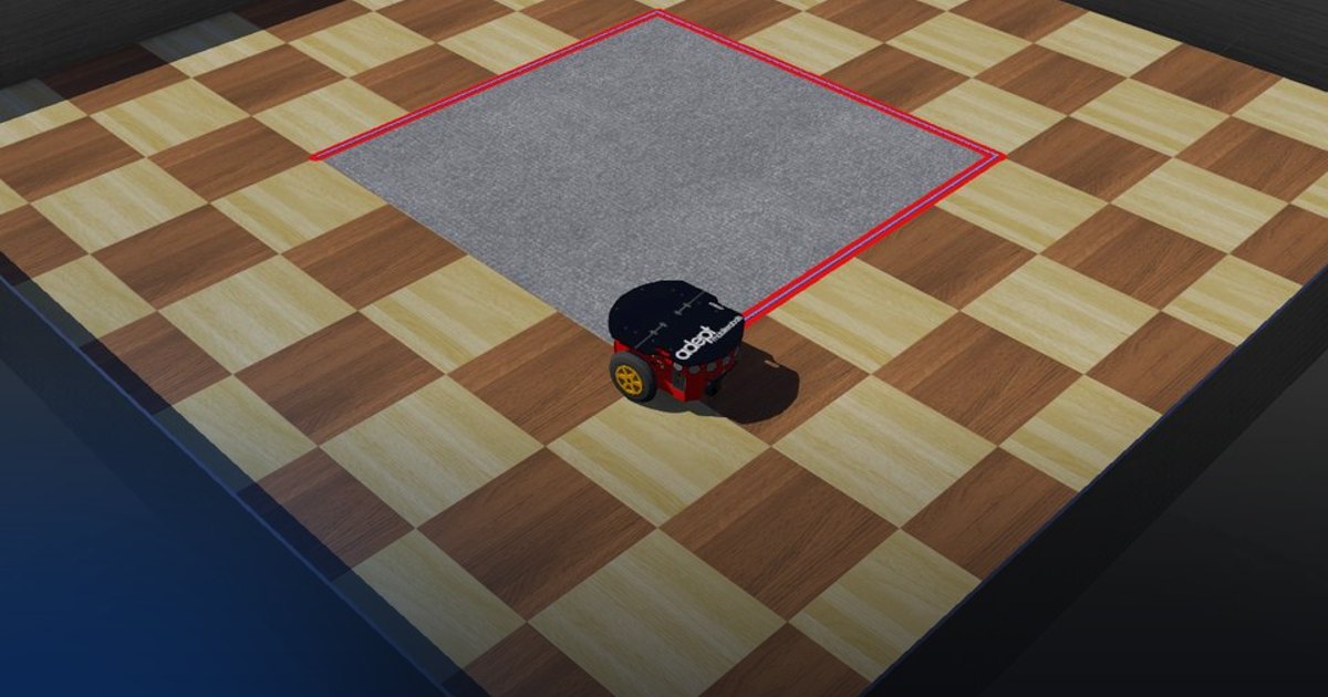
In this lesson, a Pioneer 3-DX robot must drive a 2 m × 2 m square: four straight sides of 2 m and three turns of 90° to the right, ending where it started. The robot has no camera, no line on the floor and no GPS; the only thing it knows about its motion is how far each wheel has turned, measured by the wheel encoders.
The lesson covers dead reckoning (estimating the pose by integrating the wheel motion), the differential-drive kinematic model in both directions, and two closed-loop motion primitives built on the estimate: drive a distance and turn to a heading.
Theoretical Background
Differential-Drive Kinematics
The Pioneer has two driven wheels of radius \(r\) on a common axle, a distance \(d\) apart (the wheel base), and a passive caster at the back. If the left and right wheels turn at angular speeds \(\omega_l\) and \(\omega_r\) [rad/s], their rims move at \(v_l = r\,\omega_l\) and \(v_r = r\,\omega_r\) [m/s]. The centre of the axle then moves forward with the mean of the two and rotates with their difference:
where \(v\) is the linear speed [m/s] and \(\omega\) the yaw rate [rad/s], positive counter-clockwise. Two special cases are all a square needs:
| Motion | Wheel speeds | Robot speeds |
|---|---|---|
| Straight line | \(\omega_l = \omega_r\) | \(v \neq 0\), \(\omega = 0\) |
| Turn on the spot | \(\omega_l = -\omega_r\) | \(v = 0\), \(\omega \neq 0\) |
To make the robot move with a desired \((v, \omega)\), invert the model (the inverse kinematics): each rim must move at \(v\) plus or minus the part of the rotation it carries, \(\omega\,d/2\):
Odometry
A wheel encoder reports the wheel's angle \(\theta\) [rad]. Between two control steps the left and right wheels turn by \(\Delta\theta_l\) and \(\Delta\theta_r\); if they roll without slipping, they travel the arcs
The robot centre advances by \(\Delta s\) and turns by \(\Delta\phi\):
With the pose \((x, y, \phi)\) (position in metres, heading in radians from the \(x\) axis), the update over one step uses the heading halfway through the step, the midpoint rule:
Using the old heading instead (\(\phi_k\)) is the Euler rule; it is exact for straight lines but cuts every curve slightly short. The midpoint rule is exact for an arc of constant curvature, so it is a better fit for a wheel step. \(\mathrm{wrap}\) keeps the heading in \([-\pi, \pi)\), so that the difference between two headings is always the short way round.
Integrating increments like this is dead reckoning. Its weakness is that errors never go away: a wrong wheel radius scales every distance, a wrong wheel base scales every turn, and wheel slip adds noise that the encoders cannot see. A heading error is the most damaging, because it turns into a sideways error that grows with the distance driven. After a straight run of length \(L\) with a heading error \(\delta\), the robot is off its line by
| Heading error \(\delta\) | Sideways error after one 2 m side |
|---|---|
| 0.5° | 1.7 cm |
| 1° | 3.5 cm |
| 3° | 10.5 cm |
| 5° | 17.4 cm |
and on a square these errors add up from side to side. This is why the old robotbenchmark version of this challenge, which drove for a fixed time instead of measuring the motion, is so sensitive: a timing error of a few milliseconds at each corner is already a degree.
Motion Primitives
The square is a plan of seven moves, each one a primitive with its own target, done one after the other:
stateDiagram-v2
    direction LR
    [*] --> Side1
    Side1 --> Turn1: 2 m driven
    Turn1 --> Side2: heading -90°
    Side2 --> Turn2: 2 m driven
    Turn2 --> Side3: heading 180°
    Side3 --> Turn3: 2 m driven
    Turn3 --> Side4: heading 90°
    Side4 --> [*]: 2 m driven, stop
Drive a distance. Let the side start at \((x_s, y_s)\) and run along the heading \(\phi_d\). The distance covered so far is the projection of the displacement onto the side's unit vector, so that a sideways drift does not count as progress:
The remaining distance \(e_s = L - s\) sets the speed through a proportional law with saturation, and a second proportional term keeps the heading on the side's direction:
\(\mathrm{sat}(u; a, b)\) keeps the sign of \(u\) and limits its magnitude to \([a, b]\). The upper limit is the cruise speed; the lower one keeps the robot from crawling forever as \(e_s \to 0\) (a pure proportional law only approaches the target asymptotically). Far from the corner the robot cruises at \(v_{\max}\); within \(v_{\max}/K_s\) of it (0.4 m with the default gains) it slows down linearly, so it arrives at the corner almost at rest instead of overshooting. The move ends when \(e_s\) falls below a small tolerance.
Turn to a heading. On the spot (\(v = 0\)), the heading error drives the yaw rate in the same way:
and the move ends when \(|\mathrm{wrap}(\phi_d - \phi)|\) is below the angle tolerance.
Absolute headings. The target heading of side \(k\) is \(\phi_k = k \cdot (-90°)\) relative to the start, not "the current heading minus 90°". If a turn ends 0.2° short, the next straight segment's heading term corrects it instead of carrying the error into every later side. Both primitives are feedback loops on the estimate: they make the estimated pose do the right thing, and the real robot follows as well as the odometry is right.
Task Description
Objective
Implement the functions marked IMPLEMENT HERE in controllers/square_path/square_path.py:
get_wheel_travel: the distance each wheel rolled since the last step, from the encoder increments.update_pose: the odometry update of \((x, y, \phi)\) with the midpoint rule.distance_along: the progress along the current side, as a projection onto its direction.straight_command: the linear and angular speed that finish a side (saturated P on distance, P on heading).turn_command: the yaw rate that turns the robot on the spot to the target heading.get_wheel_speeds: the inverse kinematics, from \((v, \omega)\) to the wheel speeds.
The plan of moves, the switching between them and the calls to the robot are already written in main().
System Configuration
- Robot: Pioneer 3-DX, differential drive, wheel radius \(r = 0.0975\) m, wheel base \(d = 0.33\) m
- Sensors:
left wheel sensor,right wheel sensor: wheel encoders, angle in rad, read withget_wheel_encoder_positions() - Actuators:
left wheel,right wheel: velocity-controlled motors, at most 5.24 rad/s (about 0.51 m/s at the rim), set withset_wheel_velocity(left, right) - Environment: a flat 5 m × 5 m arena; the robot starts at the origin facing \(+x\), and the square runs clockwise around the grey carpet: \((0, 0) \to (2, 0) \to (2, -2) \to (0, -2) \to (0, 0)\)
- Control step: 16 ms
- Visualization: a Matplotlib window (
path_plot.py) draws the planned square and the path the odometry estimates, with the estimated heading; the red pen on the robot draws the real path on the floor
Performance Metrics
A supervisor watches the robot's real position (not the controller's estimate) at every step, compares it with the
square laid out from the start pose, and writes metrics.json:
| Metric | Meaning |
|---|---|
success |
true when the robot stopped with every side at least 90 % covered and within 0.25 m of the start |
reason |
why the run ended: square completed, stopped early, left the path, did not start, time limit |
time |
simulated time when the run ended [s] |
distance_m |
length of the path driven [m] |
mean_deviation_m |
mean distance from the square, averaged over the path length driven [m] |
max_deviation_m |
largest distance from the square [m] |
side_coverage |
for each side, the fraction of its 10 cm stretches the robot passed within 0.25 m of |
coverage |
the mean of the four side coverages (0 to 1) |
return_error_m |
distance between the final and the start position [m] |
score |
\(100 \cdot \text{coverage} \cdot \max(0,\, 1 - \text{mean deviation} / 0.25\ \text{m})\) |
The mean deviation is weighted by distance, \(\bar e = \sum_k e_k\,\Delta s_k / \sum_k \Delta s_k\), so time spent turning on the spot or standing still neither helps nor hurts. The run ends when the robot has stood still for 1 s after moving, when it gets more than 0.5 m away from the square (failure), when it has not moved after 5 s (failure), or after 60 s (failure). A good solution finishes in about 40 s with a mean deviation of about a centimetre.
Suggested Algorithm
At each control step:
- Read the two encoders and compute the distance each wheel rolled since the previous step.
- Update the pose estimate \((x, y, \phi)\) with the odometry equations; remember the encoder values.
- Take the current move of the plan and compute its heading error \(\mathrm{wrap}(\phi_d - \phi)\).
- On a side: compute the remaining distance; if it is below the tolerance the move is done, otherwise compute
\((v, \omega)\) with
straight_command. - In a turn: if the heading error is below the tolerance the move is done, otherwise compute \(\omega\) with
turn_commandand keep \(v = 0\). - When a move is done, remember the current position as the start of the next side and go to the next move; after the last one, command zero speed.
- Convert \((v, \omega)\) into wheel speeds and send them to the motors.
Validation Checklist
- With the wheels stopped, the pose estimate stays exactly where it is.
- On the first side, \(x\) grows and \(y\) and \(\phi\) stay near zero; the console shows \(x \approx 2\) at the first corner.
- The heading printed after each turn is close to −90°, 180° and 90°, and never jumps by \(2\pi\) during a turn.
- The robot slows down before each corner and does not overshoot it.
- In the plot, the estimated path lies on the planned square; the red pen trace on the floor (the real path) runs along the edge of the grey carpet, with sharp corners. The two agree only as well as the odometry is right.
- The supervisor reports
success: true, a mean deviation of a few centimetres or less and a full coverage.
References
- Pioneer 3-DX in the Webots guide
- Webots PositionSensor (wheel encoders)
- Differential wheeled robot (Wikipedia)
- Dead reckoning (Wikipedia)
- R. Siegwart, I. Nourbakhsh, D. Scaramuzza, Introduction to Autonomous Mobile Robots, 2nd ed., MIT Press, 2011: §3.2 (kinematic models) and §5.2.4 (odometric position estimation and its error model)
- J. Borenstein, L. Feng, "UMBmark: A Method for Measuring, Comparing, and Correcting Dead-Reckoning Errors in Mobile Robots", University of Michigan, 1994: the square-path test used to calibrate real robots' odometry
Extension Ideas
- Change
WHEEL_BASEby a few percent and watch the square open up; then drive the square both clockwise and counter-clockwise and use the two end errors to calibrate the wheel base, as in the UMBmark method. - Replace the turn on the spot with a rounded corner: drive an arc of radius \(R\) with \(\omega = v / R\) and compare the time and the mean deviation.
- Drive to each corner as a point (distance and bearing to the goal, as in a go-to-goal controller) instead of a distance along a heading, and compare how the errors build up.