Trajectory Tracking Controller (Odometry + Kinematic Tracking)
Make an e-puck follow a planned trajectory using odometry and a kinematic tracking controller.
Free. Runs in your browser; you'll be asked to sign in first.
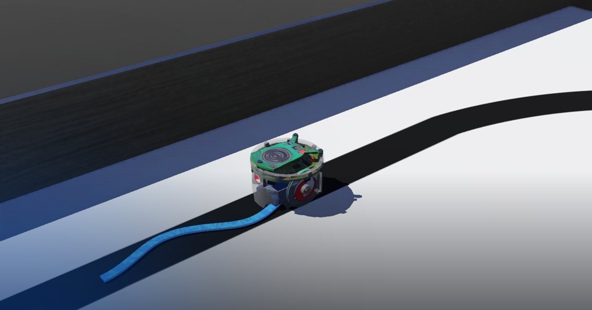
Trajectory Tracking with Odometry
Overview
In this lesson, the robot must follow a time-varying trajectory instead of moving to a single fixed goal. The controller estimates the robot pose from wheel encoders, computes the active reference trajectory, and generates wheel commands that keep the robot close to that moving target.
The lesson covers trajectory generation and kinematic trajectory tracking for a differential-drive robot.
Theoretical Background
Differential-Drive Kinematics
Wheel encoder readings yield wheel angular speeds \(\omega_l\) and \(\omega_r\). The robot linear and angular speeds are:
Point-of-Interest Motion
The tracked point is located a distance \(A\) in front of the wheel axle. Its Cartesian speeds are:
Kinematic Tracking Law
If the desired tracked-point position is \((x_d, y_d)\), define the position errors:
A common tracking law is:
These references are then converted into wheel speeds and saturated to motor limits. Kx and Ky are positive proportional tracking gains. In this lesson, use Kx = 1.0 and Ky = 1.0.
Task Description
Objective
The odometry functions (get_wheels_speed, get_robot_speeds, get_robot_pose) and wheel_speed_commands are
provided. Implement in trajectory_tracking_controller.py:
get_cartesian_speeds(u, w, phi, a): the velocity \((\dot{x}, \dot{y}, \dot{\phi})\) of the tracked point.reference_trajectory(t, x_ref0, y_ref0): the active reference trajectory below and its time derivatives.traj_tracking_controller(dxd, dyd, xd, yd, x, y, phi, a): the tracking law, returning \(u_{\text{ref}}\) and \(\omega_{\text{ref}}\).
The main loop integrates the odometry of the tracked point, evaluates the reference, runs the controller, sets the wheel speeds, and prints the distance error about twice a second.
System Configuration
- Robot: e-puck differential-drive robot (wheel speeds up to about 6.28 rad/s)
- Sensors: wheel encoders (
get_wheel_encoder_positions(), rad) - Actuators: left and right wheel motors
- Parameters (in the code): wheel radius \(R = 0.0205\) m, effective wheel separation \(D = 0.0565\) m, tracked point \(A = 0.05\) m ahead of the wheel axle
- Initial pose:
get_current_pose()gives the true starting pose once; \((x_{\text{ref0}}, y_{\text{ref0}})\) is the tracked point's starting position
Required Trajectories
For the first 15 seconds, the tracked point must follow:
with:
- \(v_1 = 0.01\) m/s
- \(A_1 = 0.03\) m
- \(w_1 = 0.4\) rad/s
For the next 15 seconds, let \(t_2 = t - 15\) and follow:
with:
- \(v_2 = 0.006\) m/s
- \(A_{x2} = 0.03\) m
- \(w_{x2} = 0.35\) rad/s
- \(A_{y2} = 0.02\) m
- \(w_{y2} = 0.70\) rad/s
For both segments, derive \(\dot{x}_d\) and \(\dot{y}_d\) from the trajectory equations and pass those values to the tracking controller.
Performance Metrics
A supervisor computes the same reference and compares it with the robot's real tracked point (from the robot's
true pose) for 30 s. The run ends early when the real tracked point is more than 10 cm from the reference
(lost_reference). It writes:
| Metric | Meaning |
|---|---|
success |
the run completed with a mean error of at most 2 cm on each trajectory and never more than 5 cm |
ended_reason |
completed or lost_reference |
time_s |
simulated time of the run [s] |
trajectory1_mean_error_m, trajectory1_max_error_m |
real tracking error on the first trajectory [m] |
trajectory2_mean_error_m, trajectory2_max_error_m |
real tracking error on the second trajectory [m] |
final_error_m |
real tracking error at the end [m] |
odometry_final_error_m |
the same error according to odometry reconstructed from the wheel encoders [m] |
smoothness |
how smooth the wheel commands were, 0 to 1 |
saturation_fraction |
fraction of the time a wheel command was at the motor limit |
score |
0 to 100, from the tracking errors of both trajectories (70%), smoothness (20%) and saturation (10%) |
Suggested Control Pipeline
At each control step:
- Read the wheel encoders and update the odometry estimate.
- Compute the tracked-point pose.
- Select the active trajectory segment from time.
- Evaluate \(x_d\), \(y_d\), \(\dot{x}_d\), and \(\dot{y}_d\).
- Compute the tracking error.
- Generate \(u_{\text{ref}}\) and \(\omega_{\text{ref}}\).
- Convert the references into wheel commands.
Validation Checklist
- The first trajectory moves forward in \(x\) and oscillates in \(y\).
- The second trajectory starts only after 15 seconds.
- The derivatives match the chosen trajectory equations.
- The distance error printed in the console stays small (about twice a second).
- The robot stays close to the reference on both segments.
References
- Motion control and velocity-based dynamic compensation for mobile robots
- Adaptive dynamic controller for trajectory tracking
- E-puck robot specifications
Extension Ideas
- Tune the controller gains for faster convergence with less oscillation.
- Try other feasible trajectories without changing the controller structure.
- Study how the tracked-point offset \(A\) affects the tracking behavior.