Visual Tracking
Make a robot dog track a moving rubber duck with its camera using color segmentation.
Free. Runs in your browser; you'll be asked to sign in first.
Overview
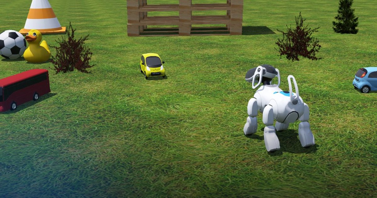
A Sony Aibo ERS-7 stands in a garden and a yellow rubber duck moves around it. The robot does not walk: it only turns its head, and the camera in its nose must keep looking at the duck for the whole run (about 100 seconds of simulated time). A supervisor checks, from the real positions in the world, how often the camera really points at the target.
The lesson covers the two halves of every vision-based controller: perception (finding the target in the image with an HSV colour threshold and computing its centroid from image moments) and visual servoing (turning the target's pixel position into angle errors with the pinhole camera model and driving the pan/tilt joints with a proportional controller).
Theoretical Background
The camera image
The camera returns an image of \(W \times H\) pixels (\(480 \times 320\) here). OpenCV stores it as an array of shape
(H, W, 3) in BGR order; pixel \((u, v)\) is column \(u\) (left to right) and row \(v\) (top to bottom), with
\((0, 0)\) in the top-left corner. The image centre is \((u_0, v_0) = (W/2,\ H/2)\).
Colour segmentation in HSV
In RGB, a colour's brightness is spread over all three channels: the sunlit and the shaded side of the same yellow duck have very different \((R, G, B)\) values. The HSV colour space separates what colour from how bright:
| Channel | Meaning | OpenCV range |
|---|---|---|
| \(H\) (hue) | the colour's angle on the colour wheel: red 0, yellow 30, green 60, blue 120 | 0–179 (degrees / 2) |
| \(S\) (saturation) | how pure the colour is: grey 0, vivid 255 | 0–255 |
| \(V\) (value) | how bright: black 0 | 0–255 |
With \(M = \max(R, G, B)\), \(m = \min(R, G, B)\) and \(\Delta = M - m\): \(V = M\), \(S = \Delta / M\), and the hue is the angle of the dominant channel, e.g. \(H = 60^\circ \cdot \frac{G - B}{\Delta}\) when \(M = R\). A shadow lowers \(V\) but barely moves \(H\), so a box in HSV catches the whole object:
The duck is a warm yellow (\(H \approx 26\)). The scene has two traps: a yellow car whose paint is a slightly greener yellow (\(H \approx 31\)) and grass that is yellow-green (\(H \approx 40\)), so the hue window must be narrow (\(20 \le H \le 28\)). A lower bound on \(S\) rejects the greyish ground and sky, and a lower bound on \(V\) rejects dark pixels, whose hue is mostly noise. Plotting the hue of a few pixels of each object is the quickest way to choose such bounds. A morphological opening (an erosion, which removes every white region smaller than the kernel, followed by a dilation, which restores the size of what survived) cleans isolated pixels.
Blobs and the centroid from image moments
The mask can contain several white regions (blobs): the duck, and perhaps something else yellow in the scene. We keep the largest one, assuming the target is the biggest yellow thing in view. The raw image moments of a region are
where \(I(u,v)\) is 1 inside the region and 0 outside. \(m_{00}\) is the area in pixels, and the centroid (the mean pixel position) is
The centroid averages many pixels, so it is far less noisy than, say, the position of the brightest pixel. A blob smaller than a minimum area is treated as noise: then the target is not visible.
From pixels to angles: the pinhole model
A pinhole camera projects a point at angle \(\theta\) from its optical axis onto the image at \(u - u_0 = f \tan\theta\) pixels from the centre, where \(f\) is the focal length in pixels. The horizontal field of view \(\alpha\) spans the half width \(W/2\) at the edge, so
With \(\alpha = 0.993\) rad (\(56.9^\circ\)) and \(W = 480\): \(f \approx 443\) px. Inverting the projection gives the angles the head must turn to centre the target (pixels are square, so the same \(f\) holds vertically):
The signs follow the robot's joints: \(e_{pan} > 0\) when the target is to the left of the centre (a positive pan turns the head left), and \(e_{tilt} > 0\) when it is above (image rows grow downwards, a positive tilt raises the head). Working in angles instead of raw pixels makes the controller gains independent of the image resolution.
Visual servoing with a proportional controller
Image-based visual servoing closes the loop through the image: the error is measured in the camera's view and the actuators move to cancel it. Here each joint is velocity controlled, so its angle \(q\) integrates the commanded speed: \(\dot q = \omega\). A proportional law
makes the error of a still target decay exponentially, since turning by \(\dot q\) changes the error by \(-\dot q\):
with time constant \(\tau = 1/K\) (\(K = 8\ \text{s}^{-1}\) gives \(\tau = 0.125\) s). When the target moves at a constant angular speed \(\dot\theta_T\) seen from the robot, the error settles at
a constant lag behind the target: a duck crossing at 0.5 m/s, 2 m away, moves at 0.25 rad/s, so \(K = 8\) leaves a lag of about \(1.8^\circ\). A larger \(K\) shrinks the lag but cannot grow without limit: the image is one control period \(T\) old when it is used, and with that delay the loop starts to overshoot as \(K T\) approaches 1 (and oscillates beyond it). With \(T = 64\) ms, \(K\) between a few and about 10 is the useful range (\(K = 8\) gives \(KT \approx 0.5\)).
graph LR
    A[Camera image] --> B[HSV threshold + opening]
    B --> C[Largest blob, centroid c_u, c_v]
    C --> D[Pinhole model: e_pan, e_tilt]
    D --> E[P controller: omega = K e]
    E --> F[Pan / tilt joints]
    F -->|head turns, the view changes| A
Task Description
Objective
Implement the four functions in visual_tracking.py:
make_target_mask(image): convert the image to HSV, threshold it withHSV_LOWER/HSV_UPPER, and clean the mask with a morphological opening.find_target(mask): find the largest blob, reject it belowMIN_AREA, and return its centroid and area from the image moments (orNone).pixel_to_angle_errors(cx, cy, width, height, fov): the pan and tilt angle errors from the pinhole model.compute_head_velocities(e_pan, e_tilt): the proportional controller withKP_PANandKP_TILT.
The main loop (Sense / Plan / Act), the behaviour when the target is lost (the head holds still), and the camera window are already written.
System Configuration
- Robot: Sony Aibo ERS-7 (
AiboErs7), standing still; only its head moves. - Sensor: the nose camera
PRM:/r1/c1/c2/c3/i1-FbkImageSensor:F1, \(480 \times 320\) pixels, horizontal field of view 0.993 rad (\(56.9^\circ\)), read every 64 ms (the control period). - Actuators (velocity mode, at most 3.01 rad/s):
- head pan
PRM:/r1/c1/c2-Joint2:12, from \(-1.62\) to \(+1.62\) rad (positive = left); - head tilt
PRM:/r1/c1/c2/c3-Joint2:13, from \(-0.35\) to \(+0.87\) rad (positive = up). - Environment: a yellow rubber duck (
DEF TARGET) moving at 0.5 m/s along a random order of seven closed paths around the robot (about 51 m, 102 s), in a garden with trees, cars, cones and pallets; the yellow car is a distractor of the same colour. - Visualization: a Matplotlib window (the Visualization tab) shows the camera image with the image centre (blue cross), the detected target (green circle, red centroid and error line), and the HSV mask.
Performance Metrics
The supervisor visual_tracking_benchmark measures, every 32 ms (each physics step), the angle between the camera's line of sight and the
direction from the head to the duck, using the real positions in the world. A step is a hit when the two unit
vectors differ by less than 0.1 in each component (roughly \(5.7^\circ\)). At the end it writes metrics.json:
| Metric | Meaning |
|---|---|
hit_rate |
hits / steps, from 0 to 1: the score |
hits, steps |
the hit count and the number of steps measured |
mean_error_deg |
the mean angle between the line of sight and the target [degrees] |
time |
simulated time at the end [s] |
completed |
true when the target ran its whole path |
success |
true when the path was completed with hit_rate \(\ge 0.8\) |
The run ends when the target's path is finished, or earlier, as a failure, when the target stays outside the camera's field of view for 10 s, or when the head has not turned at all (less than \(1^\circ\)) in the first 5 s, since the target moves from the start.
Suggested Algorithm
At each control step:
- Read the camera image.
- Convert it to HSV and threshold it into a mask; apply an opening.
- Find the external contours of the mask; keep the largest; compute its moments.
- If its area is at least
MIN_AREA, take the centroid \((c_u, c_v)\); otherwise the target is lost: stop the head. - Compute \(f\) from the field of view and the angle errors \(e_{pan}\), \(e_{tilt}\).
- Compute \(\omega_{pan} = K_{pan} e_{pan}\) and \(\omega_{tilt} = K_{tilt} e_{tilt}\) and send them to the joints.
- Update the camera window.
Validation Checklist
- The mask shows the duck as one solid white blob and little else; the ground and trees stay black.
- The green circle sits on the duck in the camera view.
- When the duck is left of the centre, the head turns left (and up when it is above): the error line shrinks.
- The duck stays near the blue cross while it moves, slightly behind it in the direction of motion (the lag \(\dot\theta_T / K\)).
- The head does not oscillate around the target; if it does, the gains are too high.
- The console's
e_panande_tiltstay within a few degrees, and the finalhit_rateis above 0.8.
References
- Webots: Sony Aibo ERS-7
- Webots: Camera
- OpenCV: Changing colour spaces (HSV thresholding)
- OpenCV: Contour features and moments
- Image moments (Wikipedia)
- Pinhole camera model (Wikipedia)
- Visual servoing (Wikipedia); F. Chaumette and S. Hutchinson, "Visual servo control, Part I: Basic approaches", IEEE Robotics & Automation Magazine, 2006.
Extension Ideas
- Remove the lag: estimate the target's angular speed from consecutive errors and add it as a feed-forward term, \(\omega = K e + \hat{\dot\theta}_T\) (or add an integral term).
- Search when the target is lost: sweep the pan joint slowly instead of holding still, and resume tracking when the duck reappears.
- Make the detection more selective: reject blobs whose size or shape (aspect ratio, fill ratio) does not match a duck, or prefer the blob closest to the last known position, so the yellow car can never steal the track.