Wall Following

Wall Following with Sonars and PD Control

Overview

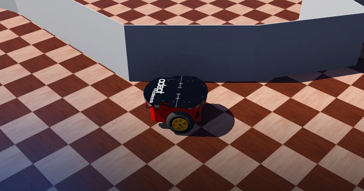
A Pioneer 3-DX starts in an arena facing a long, winding wall. It must drive up to the wall, turn so that the wall is on its left, and then follow it while keeping its centre 0.5 m away from it: along gentle bends, into inner corners where the wall turns into its path, and around outer corners where the wall turns away.

The lesson combines range sensing with feedback control: converting raw sonar readings into distances, filtering their noise, estimating the robot's distance and angle to the wall from two sensors, steering with a proportional-derivative (PD) controller, and handling corners with a small state machine.

Theoretical Background

Sonar Range Sensing

The Pioneer carries 16 ultrasonic sonars (so0 to so15) on a ring around its body. A sonar emits a sound pulse and measures the time until the echo returns; Webots turns that time into a reading through the sensor's lookup table, which here is linear: 1024 for an obstacle touching the sensor and 0 at the maximum range \(d_{max} = 5\) m. Inverting the table gives the distance

where \(v\) is the raw reading. A reading of 0 means that no echo came back: there is nothing within range in the direction the sonar can see, so the distance is taken as \(d_{max}\).

Sound reflects off a flat wall like light off a mirror (specular reflection). A sonar only hears its echo when its beam hits the wall nearly head-on: in this simulation, when the angle of incidence (between the beam and the wall's normal) is below \(22.5°\). A sonar looking at a wall at a grazing angle sees nothing, even when the wall is close. This is why a wall follower needs sensors pointing in several directions, and why "the side sonar lost the wall" can mean two different things: the wall turned away (an outer corner), or the wall turned towards the robot so that the side beam now grazes it (an inner bend, which the forward-looking sonars see).

Filtering the Noise

Each reading carries Gaussian noise with a standard deviation of 1 % of the raw value, about 4 to 5 cm at the distances that matter here. A first-order low-pass filter (an exponential moving average) smooths it:

where \(d_k\) is the new measurement and \(\hat d_k\) the filtered estimate. With \(\alpha = 1\) there is no filtering; smaller values remove more noise but react later: the filter's time constant is about \(\tau \approx \Delta t / \alpha\) (with the control period \(\Delta t = 16\) ms and \(\alpha = 0.3\), about 50 ms). For white noise the filter divides the standard deviation by \(\sqrt{(2 - \alpha)/\alpha}\), about 2.4 for \(\alpha = 0.3\).

The sonar's errors are not symmetric, though. Besides the small Gaussian noise, a sonar often misses an echo (the beam grazed a wall, or the robot turned for a moment): the reading jumps to the full 5 m. It hardly ever reports an obstacle that is not there. A robot that trusts every "nothing here" reading drives into walls it saw a moment ago, so the filter uses two factors: a large one (\(\alpha_{closer} = 0.5\)) when the reading is closer than the estimate, and a small one (\(\alpha_{farther} = 0.1\)) when it is farther:

A single missed echo now moves a 0.5 m estimate only to 0.95 m, while an obstacle that appears is taken in at once. A wall that really disappears (an outer corner) still shows within two or three steps, because the jump is large.

Distance and Angle to the Wall

Two sonars on the same side, so0 in front and so15 behind, a baseline \(L = 0.216\) m apart and both pointing perpendicular to the robot, measure two ranges \(d_f\) and \(d_r\) to a straight wall. If the robot is parallel to the wall, \(d_f = d_r\); if its nose points towards the wall by an angle \(\theta\), the front range is shorter:

The perpendicular distance from the robot's centre to the wall is the mean range plus the sensors' lateral offset \(o = 0.14\) m from the robot's centre line, projected onto the wall's normal:

When the rear sonar sees nothing (just after an outer corner), or the two ranges differ by more than \(L\) (an angle above \(45°\): at a corner the two sonars see two different walls), the best guess is that the robot is parallel to the wall the front sonar sees: \(\theta = 0\) and \(d = d_f + o\).

PD Control of the Distance

The error is how much farther from the wall the robot is than the target \(d^* = 0.5\) m:

With the wall on the left, a positive error means "turn left", a positive (counter-clockwise) turning rate \(\omega\). A proportional controller alone, \(\omega = K_p e\), keeps turning towards the target line until it reaches it, arrives there at an angle and overshoots: the robot weaves along the wall. The derivative term damps the motion by reacting to how fast the error changes:

Differentiating the noisy distance numerically, \(\dot e \approx (e_k - e_{k-1})/\Delta t\), divides 1 to 2 cm of noise by 16 ms: the derivative would be mostly noise. Geometry gives it directly instead. Moving at speed \(v\) with the nose at the angle \(\theta\) towards the wall, the distance shrinks at

so the PD law becomes

and \(\omega\) is limited to \(\pm\omega_{max}\) so that a large error never makes the robot spin. Near the target this is a linear second-order system: with \(\dot\theta = \omega\) and \(\sin\theta \approx \theta\), \(\ddot e = -v\,\dot\theta = -v\,(K_p e + K_d \dot e)\), that is

with the natural frequency \(\omega_n = \sqrt{v K_p}\) and the damping ratio \(\zeta = \dfrac{K_d}{2}\sqrt{\dfrac{v}{K_p}}\). With \(v = 0.4\) m/s, \(K_p = 2\) and \(K_d = 4\): \(\omega_n \approx 0.89\) rad/s and \(\zeta \approx 0.89\), a quick response with almost no overshoot. Without the D term (\(K_d = 0\)) the damping is zero and the robot oscillates around the target line forever.

Differential-Drive Kinematics

The controller decides a linear speed \(v\) and a turning rate \(\omega\); the motors take wheel speeds. For wheels of radius \(R = 0.0975\) m that are \(D = 0.33\) m apart, each wheel's rim moves at the robot's speed plus or minus the rotation's share at the distance \(D/2\):

Corners: a State Machine

The PD controller follows a wall whose direction changes slowly. Sharp corners need different behaviours:

stateDiagram-v2
    [*] --> FIND_WALL
    FIND_WALL --> INNER_CORNER: wall ahead
    INNER_CORNER --> FOLLOW: ahead clear and left sonar sees the wall
    FOLLOW --> INNER_CORNER: wall ahead, or so1 sees the wall bending in
    FOLLOW --> OUTER_CORNER: left sonar lost the wall
    OUTER_CORNER --> FOLLOW: left sonar sees the wall again
    OUTER_CORNER --> INNER_CORNER: wall ahead

• FIND_WALL: drive straight until the wall is ahead.
• INNER_CORNER (the wall turns into the robot's path): turn right on the spot, \(v = 0\), \(\omega = -\omega_{turn}\), until the way ahead is clear and the left sonar sees the wall.
• OUTER_CORNER (the wall turns away): drive on a circle of radius \(d^*\) around the corner, \(v = v_c\), \(\omega = v_c / d^*\), until the left sonar sees the new wall.
• FOLLOW: the PD controller.

The checks for a wall ahead come before the check for a lost wall: when the wall bends towards the robot, the side sonar loses it too (its beam now grazes the new segment), and turning left there would drive into it.

Task Description

Objective

Implement the functions marked IMPLEMENT HERE in wall_following.py:

1. sonar_to_distance: convert a raw sonar reading into metres.
2. low_pass: filter the readings with the asymmetric first-order low-pass filter.
3. estimate_wall: compute the distance and the angle to the wall from so0 and so15.
4. pd_steering: compute the turning rate with the PD law above.
5. choose_state: the corner state machine.
6. wheel_speeds: convert \(v\) and \(\omega\) into wheel speeds.

The loop in main() (sense, plan, act) and the robot wrapper are given. Once it runs, tune the gains and thresholds.

System Configuration

• Robot: Adept Pioneer 3-DX, differential drive, wheel radius \(R = 0.0975\) m, wheel separation \(D = 0.33\) m, maximum wheel speed 5.24 rad/s (about 0.51 m/s).
• Sensors: 16 sonars so0 to so15, range 0 to 5 m, raw readings 0 to 1024, 1 % noise, \(22.5°\) incidence limit. The student's code uses so0, so1, so2 to so6 and so15.
• Actuators: the left and right wheel motors (velocity control).
• Control period: 16 ms.
• Environment: a wall of 46 one-metre segments with bends from \(15°\) to \(135°\), inner and outer. The robot starts 4.5 m in front of the wall, facing it, and follows it with the wall on its left.

Performance Metrics

A supervisor tracks the robot's true position and its contacts. It ends the run when the robot has followed 25 m of wall (success), touches a wall with its body, makes no progress for 15 s, moves more than 2 m away from the wall, or reaches the 120 s limit, and writes:

Progress counts only along the wall, segment by segment: cutting across to a later part of the wall does not count. The solution follows the 25 m in about 80 s with a mean distance error of about 6 to 7 cm.

Suggested Algorithm

At each control step:

1. Read the 16 sonars and convert each reading into metres.
2. Low-pass filter the distances.
3. Take the distance ahead (the smallest of so2 to so6), so1, and the left pair so0 and so15.
4. Choose the state with the state machine.
5. Estimate the distance and the angle to the wall.
6. Choose \(v\) and \(\omega\) for the state (the PD controller in FOLLOW).
7. Convert them into wheel speeds and send them to the motors.

Validation Checklist

• With the robot parallel to the wall, estimate_wall gives an angle near 0 and a distance near the true one.
• The robot turns right in front of the wall and leaves INNER_CORNER with the wall on its left.
• Along a straight segment the distance settles near 0.5 m without weaving.
• At an inner corner the robot turns on the spot; at an outer corner it drives around the corner's end.
• The printed states match what the robot is doing.
• The supervisor reports success with a small mean_distance_error_m.

References

• Pioneer 3-DX in Webots
• Webots DistanceSensor (sonar type, lookup tables)
• PID controller
• Exponential smoothing
• R. Siegwart, I. Nourbakhsh, D. Scaramuzza, Introduction to Autonomous Mobile Robots, 2nd ed., MIT Press, 2011: chapter 3 (kinematics) and chapter 4 (range sensors).

Extension Ideas

• Use more sonars to estimate the wall's angle (a line fitted through several echoes) instead of only so0 and so15.
• Slow down before corners and speed up on straight segments to follow the wall faster.
• Plot the true and the estimated distance over time (Matplotlib) to see the filter's lag and the PD controller's damping; try \(K_d = 0\).
• Empty the wall's angles field in the world: the LinkedWalls PROTO then builds a random wall on every run. Does your controller still work?